Volume raycaster (3D iso-surfaces and DVR)
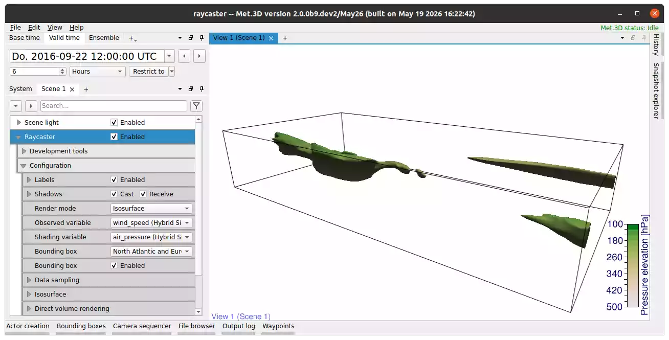
Fig. 28 Volume iso-surface actor, together with a transfer function.
Description
The volume raycaster actor visualizes 3-D scalar fields using either iso-surface raycasting or direct volume rendering (DVR). The actor supports interactive exploration of atmospheric simulation data and provides advanced illumination and shadowing techniques.
Rendering of multiple iso-surfaces from a scalar field.
Independent colouring of iso-surfaces by a second scalar field (e.g. wind-speed iso-surfaces coloured by temperature).
Shadow casting of iso-surfaces and normal curves onto other scene actors.
Rendering of normal curves on iso-surfaces.
Interactive region-contribution analysis for iso-surfaces.
Direct volume rendering of up to three scalar fields simultaneously.
Optional volumetric lighting approximating physical light transport.
Volumetric shadow casting onto other scene geometry.
Atmospheric cloud rendering based on liquid and ice water optical thickness.
Render mode and rendered variables
The rendering behaviour of the actor is controlled by the Render mode property. The following rendering modes are available:
Isosurface rendering
Bitfield
Direct volume rendering
Direct volume rendering with volumetric lighting
For iso-surface and bitfield rendering, the following variables are available:
- Observed variable
Scalar field from which the iso-surfaces are extracted.
- Shading variable
Optional scalar field used to colour the iso-surface.
For direct volume rendering, up to three scalar variables can be rendered simultaneously:
- Observed variable
Scalar field used as the primary DVR volume.
- Second variable
Optional secondary scalar field rendered together with the primary volume. Located under the direct volume rendering settings.
- Third variable
Optional tertiary scalar field rendered together with the primary volume. Located under the direct volume rendering settings.
- Shading variable
Optional scalar field used for cloud colouring and shading.
The transfer function for each variable determines how it contributes to colour and opacity.

Iso-surface rendering
Iso-surface rendering extracts surfaces of constant scalar value from the observed variable. Multiple iso-values can be rendered simultaneously.
Each iso-surface can be configured independently with respect to:
Iso-value
Colour mode
Surface colour
Opacity
Optionally, the iso-surface colour can be derived from a second scalar field using the shading variable and its associated transfer function.
The actor supports shadow casting of iso-surfaces onto other geometry in the scene. Shadowing improves depth perception and spatial interpretation of complex atmospheric structures.
Normal curves
Met.3D can render normal curves between two iso-surfaces. Alternatively, the curve length can be limited by specifying the maximum number of line segments. Normal curves can be rendered as tubes, lines, or box-and-slice glyphs. The user can also set the seed point spacing.

Bitfield rendering
Similar to iso-surface rendering, but instead of a variable visualizes a bitfield.
Direct volume rendering
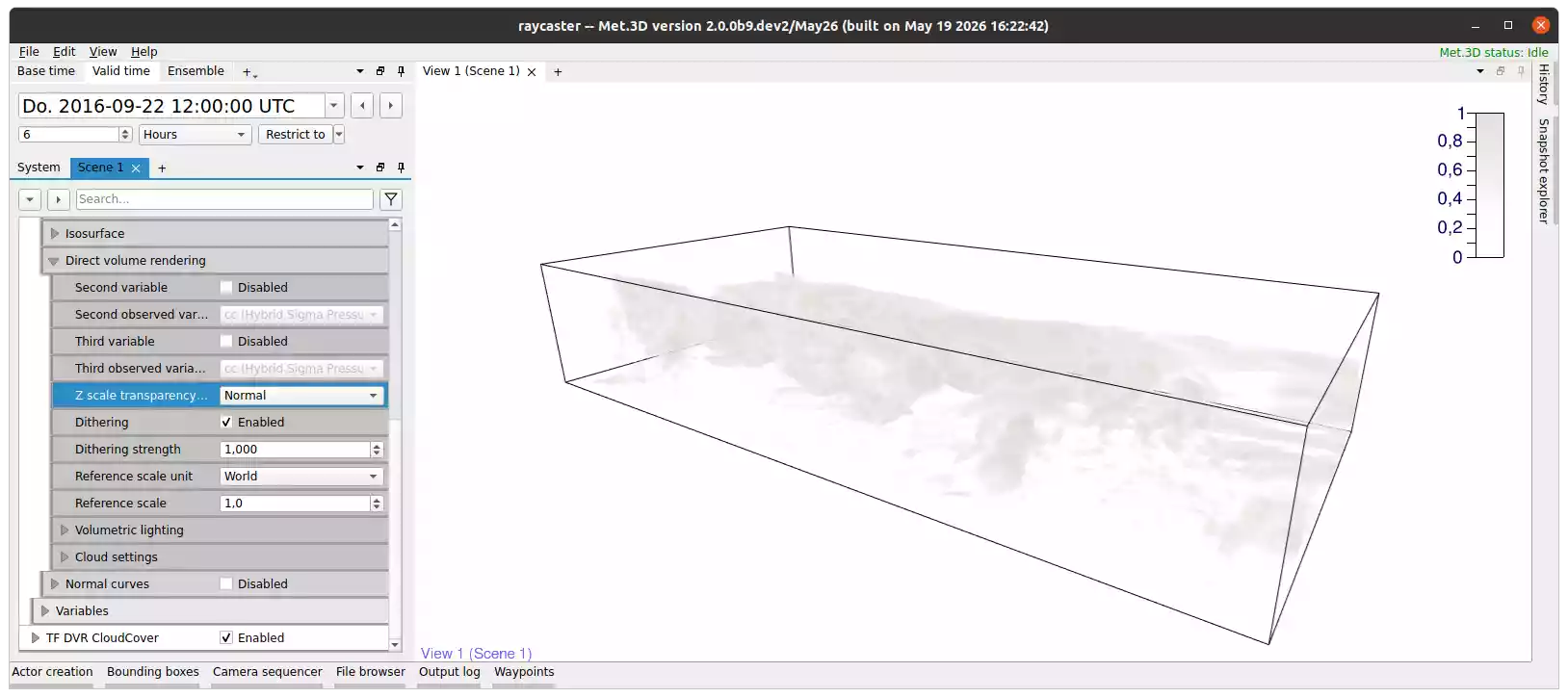
Fig. 29 A DVR scene showing the cloud cover variable.
Direct volume rendering (DVR) visualizes the full volumetric scalar field without extracting explicit surfaces.
The rendered appearance is controlled by transfer functions that map scalar values to colour and opacity. Up to three variables can be rendered simultaneously, enabling combined visualization of multiple atmospheric quantities.
Internally, alpha or transparency of the transfer function is converted to extinction coefficients. This way, we can blend the different volumes together, especially if combined with Cloud rendering.
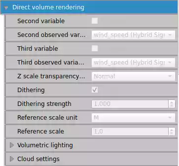
Fig. 30 Properties of the direct volume rendering mode
The following options control the DVR rendering behaviour:
Dithering – Randomizes the ray start positions slightly to avoid patterns visible with low ray step sizes.
Z scale transparency fix – Changes how transparency is affected by the scenes vertical scaling. Using the
Normaloption will only affect transparency on the z-axis, while thePhysicaloption affects all axis. Compensates for vertical scene scaling by adjusting extinction coefficients such that the resulting optical thickness remains approximately constant.Reference scale – The reference scale used when converting the alpha value of a transfer function to an extinction coefficient.
Volumetric lighting
The volumetric lighting mode approximates physical light transport through the participating medium.
The renderer casts rays from each lightmap voxel towards all light sources in the scene. The optical depth along the ray is used to compute light attenuation. Since multi-scattering is rather expensive, approximations have been implemented to emulate the effect.
Volumetric shadows generated by the volume can additionally be projected onto other scene actors.
Due to the increased computational complexity, volumetric lighting requires substantially more rendering time than standard DVR. Lighting does not need to be recomputed every frame. As a result, volumetric lighting primarily introduces an initial preprocessing cost with comparatively low runtime overhead.
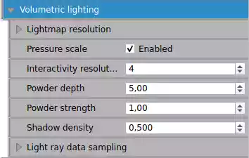
Fig. 31 Properties for volumetric lighting.
The following options control the calculation and accuracy of the volumetric lighting:
Lightmap resolution – The size of the volumetric lightmap. Higher resolutions yield more accurate results and are more expensive.
Pressure scale – Distributes the volumetric lightmap logarithmically along the vertical axis, to align better with data fields.
Interactivity resolution – Downscales the lightmap resolution during interaction with light sources for quick preview.
Powder depth – An approximation of multi-scattering resulting in darker, thin volumes. This is the depth of the effect.
Powder strength – The strength of the powder effect.
Shadow density – A multiplier to the darkness of shadows produced by the volume.
Cloud rendering
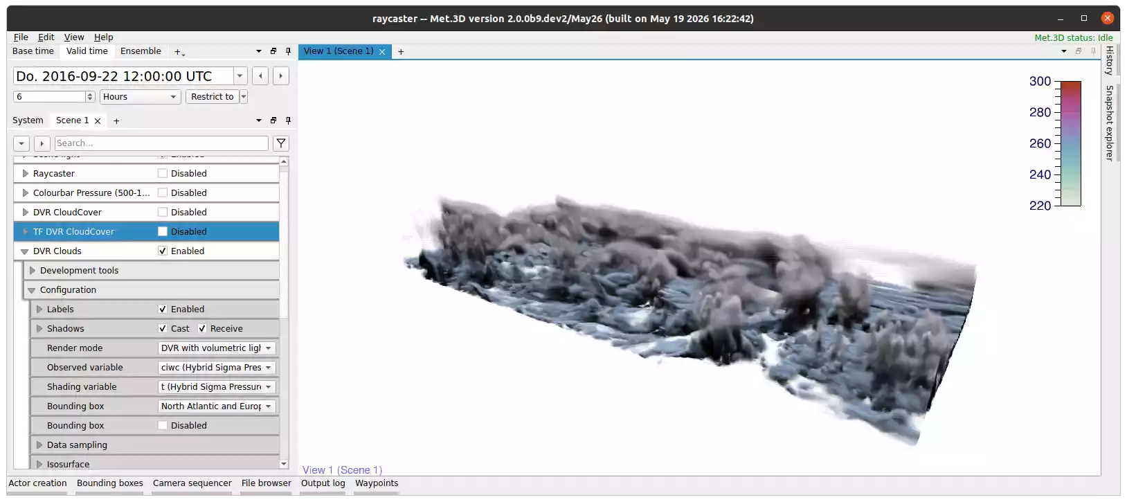
Fig. 32 A DVR scene utilizing atmospheric cloud rendering and volumetric lighting.
The actor provides a dedicated atmospheric cloud rendering mode based on liquid water and ice water optical thickness.
These options are intended for the visualization of large-scale cloud structures in numerical weather prediction and atmospheric research datasets.
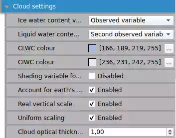
Fig. 33 Properties for atmospheric cloud rendering. Cloud liquid water content coloured in blue.
The following options control the atmospheric cloud rendering:
Ice water content variable – The variable that provides the cloud ice water content.
Liquid water content variable – The variable that provides the cloud liquid water content.
CLWC colour – The colour to use for cloud liquid water content. Can be used to differentiate both cloud variables.
CIWC colour – The colour to use for cloud ice water content. Can be used to differentiate both cloud variables.
Shading variable for cloud colour – Uses the shading variable to colour the clouds.
Account for earth’s curvature – Applies a correction to the optical thickness due to earth’s curvature.
Real vertical scale – Use the real atmospheric height in meters when calculating distances in the volume. Otherwise, uses the length of one degree longitude at the equator in meters for one unit on the vertical axis.
Uniform scaling – Applies the vertical scale onto all axis. Meaning one unit on the vertical axis is the same distance in meters as one degree longitude and latitude. Produces inaccurate clouds, but is more visually uniform.
Direct volume rendering of radar data
Example and suitable settings for rendering radar data with DVR:
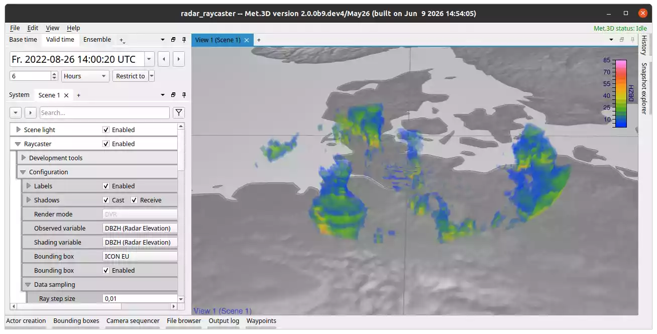
Fig. 34 Settings used: step size=0,01, interaction ray step size=0,01, use dithering=true, dithering strength=1, reference scale unit=World, reference scale=4
Multiple datasets (radar sites) can be shown at the same time in a scene either by adding multiple actors or by rendering multiple variables within the same actor.
Data sampling
The actor provides several properties to control the accuracy and performance of the raycasing. They influence how rays traverse the volume and how precisely iso-surfaces are located.
The following properties control the data sampling:
Ray step size – The distance covered by a ray per integration step in graphics space. Smaller values increase accuracy and reduce artifacts, but also increase render time.
Interaction ray step size – The ray step size used while interacting with the scene, e.g. camera movement. This value should be larger than the ray step size, to improve rendering time at the cost of accuracy during interaction.
Isosurface bisection steps – Controls the accuracy of finding iso-surface intersections along the ray. When a ray detects an iso-surface, the exact position is determined using iterative bisection of the last ray step.
Interaction isosurface bisection steps – The number of bisection refinement steps used during interaction.