Trajectory actor

Fig. 38 Trajectory actor, displaying trajectories computed in Met.3D on-the-fly, fulfilling an ascent criterion, together with a transfer function.

Description

The trajectory actor computes and renders Lagrangian particle trajectories (path lines) or streamlines as 3-D tubes or particle spheres. Trajectories can either be loaded from precomputed NetCDF files or computed on the fly from gridded wind fields. Flexible seed point sources and a multi-stage filter pipeline allow focussed visual analysis of specific trajectory subsets. Five render modes and colour modes include colouring by pressure, elapsed time, or any auxiliary variable traced along the trajectories.

Precomputed trajectories

Set Computation source to Precomputed. Under Precomputation settings, click Select data source to choose a loaded trajectory dataset. If no datasets are available, check that the trajectory NetCDF files have been loaded correctly; see Loading precomputed trajectory datasets and Trajectory data for details on loading and the expected file format.

Auxiliary variables stored in the NetCDF file (marked with attribute auxiliary_data = "yes") are automatically available for colour mapping.

Trajectories computed in Met.3D

Set Computation source to Computed within Met.3D. The following must be configured before trajectories can be computed:

1. Assign the three wind components under Computation in Met.3D: Eastward component (m/s), Northward component (m/s), and Vertical component (Pa/s).

2. Select Line type: Trajectories (path lines) or Streamlines.

3. Add at least one seed point source (see below).

4. Configure integration times and parameters (see below).

Note

On-the-fly trajectory computation runs on the CPU and requires all time steps needed for integration to fit in main memory. Start with a short integration time and increase gradually while monitoring the progress bar and console output.

Time synchronization

Three time properties control which data is loaded and which particle positions are displayed:

Base time

The forecast initialisation time. Normally synced to the session’s base time control.

Trajectory start

The time at which trajectories start integrating. For on-the-fly computation, changing this time triggers a recomputation from the new start. By default, synced to the valid time control so that advancing the valid time slider automatically restarts trajectories from the new time step.

Particle positions

The time step at which particle spheres are shown. Only relevant for render modes that display single-time positions (see below). By default, also synced to the valid-time control.

Tip

Animating particle positions along fixed trajectories: Set the Trajectory start time control to None (no synchronization). The trajectories are then computed once and held fixed. Advance the valid time control to move the Particle positions through the trajectory and watch particles travel along the path. This works with any render mode that shows single-time positions.

Ensemble

Ensemble member selects a single ensemble member. Use Synchronize with to link this actor to a session ensemble control so that the selected member follows the shared ensemble selection.

On-the-fly computation settings

Integration

Integration method

Euler (3 iter.) or Runge-Kutta (4th order).

Interpolation method

as LAGRANTO v2 follows the same interpolation as the LAGRANTO model and is recommended for reproducibility. trilinear (in lon-lat-lnp) is an alternative.

Sub-steps per data time step

Number of integration sub-steps between two wind field time steps (default 12, matching LAGRANTO v2). Higher values increase accuracy at the cost of computation time.

Backward / Forward integration time

Duration to integrate backward and forward from the trajectory start time. At least 4 vertices are required for trajectories to be visible; if integration time is very short, increase sub-steps or integration duration.

Generate vertices for each integration step

When enabled, a vertex is stored at every integration sub-step, producing smooth tubes. When disabled, vertices are only stored at wind-field time steps, which is sufficient for most purposes and saves memory.

Streamline-specific

For streamlines, configure the Streamline delta S (step length for numerical integration) and Streamline length (total number of integration segments) instead of integration time.

Integrate both base and valid time

Note

Enable Integrate both base and valid time when the wind dataset uses analysis or reanalysis data where the initialisation time equals the valid time (IT = VT). In that case the model advances both the base time and the valid time together during integration, correctly following the changing wind fields. Met.3D shows a warning if your dataset appears to have IT = VT and the option is not enabled, or vice versa.

Seed point sources

Seed points define where trajectories start. Add a source via Add seed source in the Seed points (starting positions) group. Multiple sources can be active simultaneously. Available sources:

• Horizontal cross-section actor: seeds are placed on a regular lat/lon grid at the section’s pressure level. Spacing is configurable.

• Vertical cross-section actor: seeds are placed along the section path, with configurable horizontal and pressure spacing.

• Movable pole actor: seeds are placed along the vertical axis of the pole with configurable pressure spacing.

• Bounding box: seeds are distributed on a regular 3-D lat/lon/pressure grid within the bounding box, with configurable spacing in all three directions.

In interaction mode (double-click in the scene view), any actor-based seed source can be grabbed and moved; the trajectories recompute as the source is dragged.

Seed point filters

Point filters are applied to the seed points before trajectory computation. Add a filter with Add point filter:

• Bounding box filter: retains only seed points inside a selected bounding box.

• Threshold filter: selects a gridded data variable and retains only seed points where the variable value falls within a specified lower and/or upper threshold.

Multiple filters of the same type can be added and chained.

Trajectory filters

Trajectory filters are applied after trajectories are available and work for both precomputed and computed trajectories. Add a filter with Add trajectory filter in the Trajectory filters group.

Bounding box filter

Retains trajectories that pass through a selected bounding box at any point in time.

Ascent/descent filter

Retains trajectories that ascend or descend by at least Δp hPa within a specified time window Δt. The direction criterion can be set to Ascent, Descent, Either, or Both. A typical setting for warm conveyor belts (WCBs) is 600 hPa ascent in 48 hours; see our publication on WCB analysis.

Thin-out filter

Reduces the number of trajectories by keeping every n-th trajectory along each axis of the start grid (stride in longitude, latitude, and pressure level). Useful for reducing visual clutter without changing integration or filtering logic. Only has an effect when the trajectories were started from a gridded source.

Rendering

Render mode

Set in the Rendering group via Render mode:

• Entire trajectories as tubes: full 3-D tube from start to end of each trajectory.

• All particle positions: a sphere at every stored vertex of every trajectory.

• Single time positions: spheres at the time step selected by the Particle positions property. Use this with the time animation described above.

• Tubes and single time positions: tubes plus a sphere at the current particle time. Useful for tracking individual particle positions along the full path.

• Backward tubes and single time positions: shows only the part of the tube that lies before the current particle time, giving a trailing-path effect.

Tube radius and Sphere radius control the size of the respective geometry. A warning is shown if the sphere radius is smaller than the tube radius, as spheres may then be hidden inside the tubes.

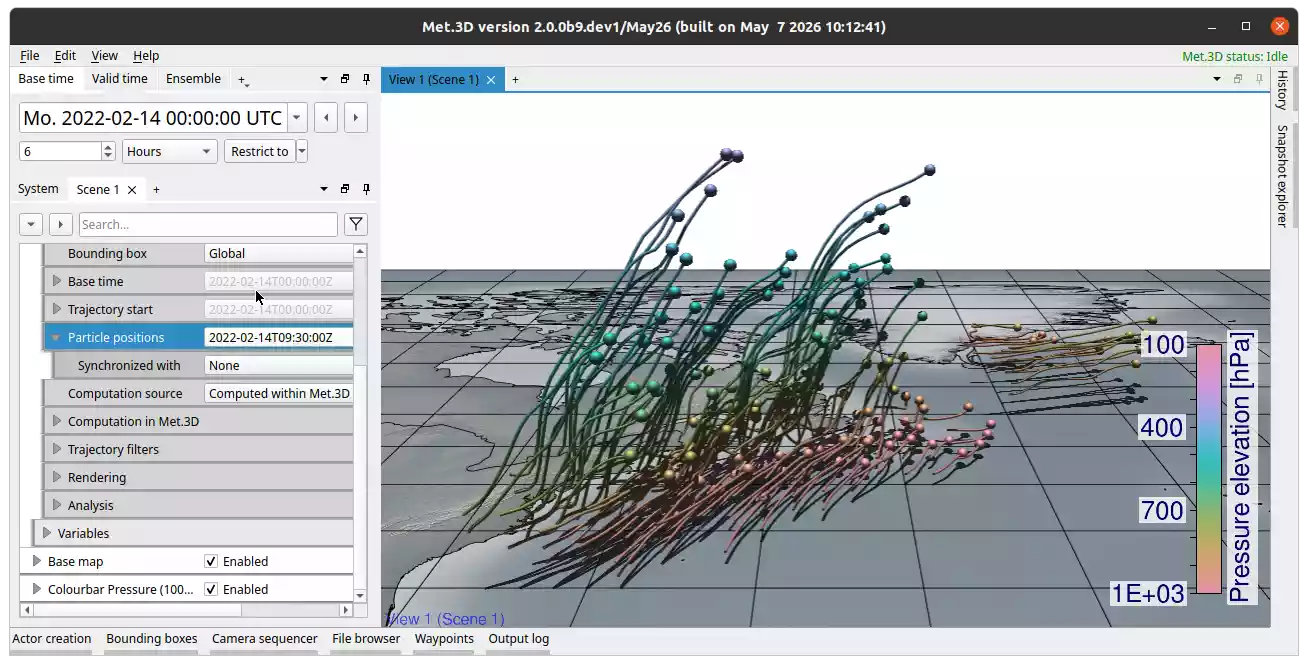
Fig. 39 Render mode Backward tubes and single time positions. You can select the particle position time in the corresponding property. This gives the visualisation a trailing-path effect.

Colour mode

Set via Colour mode:

• Constant: uniform colour set by the Colour property.

• Map pressure (hPa): colour encodes the pressure level at each vertex via the selected Transfer function.

• Map variable: colour is sampled from an auxiliary variable (selected via Mapped variable) via the transfer function. For precomputed trajectories, the variable must be present in the NetCDF file with auxiliary_data = "yes". For computed trajectories, the variable must be set as an actor variable.

• Time (hours since start): colour encodes elapsed time since the trajectory start via the transfer function.

• Time (seconds since start): same as above in seconds.

Analysis output

The Analysis group provides buttons to export data in LAGRANTO-compatible formats:

• Output as LAGRANTO ASCII exports the trajectory data.

• Output seed points as LAGRANTO start file exports the current seed points.

• Output seed points as LAGRANTO job file exports a job file for submission to a LAGRANTO FTP service.

Note

For an overview of the internal trajectory pipeline architecture (point sources, point filters, trajectory filters, and data flow), see the developer documentation: Trajectory Pipeline.