Isosurface intersection
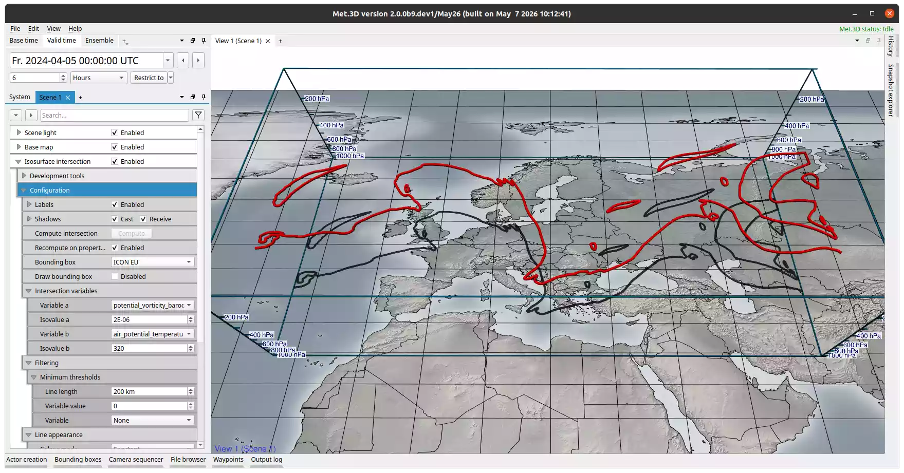
Fig. 25 Isosurface intersection actor with a bounding box. Visualized is the intersection of the 2 PVU isosurface and 320 K surface of potential temperature in the ICON-EU domain.
Description
The isosurface intersection actor computes and renders the 3-D lines where two isosurfaces of different scalar fields cross each other. Any two variables defined on the same 3-D grid can be used.
A typical meteorological application is the intersection of the 2-PVU potential vorticity isosurface with a potential temperature isosurface. The resulting lines delineate the extratropical tropopause in three dimensions and can be used to study features such as PV streamers and cutoffs (Wernli & Sprenger 2007; Kunz et al. 2015).
Setup
Under Intersection variables, select:
Variable a and its Isovalue a: the first scalar field and the isosurface value to extract from it.
Variable b and its Isovalue b: the second scalar field and its isovalue.
Both variables must be on the same 3-D grid. The intersection is computed cell by cell across the volume defined by the bounding box.
By default, Recompute on property change is enabled: the intersection is recomputed automatically whenever a variable, isovalue, or filter setting changes. Disable this and use the Compute intersection button to trigger computation manually. This is useful when experimenting with isovalues on large domains where each recomputation is slow.
Filtering
The Filtering group provides two filters under Minimum thresholds that discard short or weak line segments before rendering:
- Line length
Removes line segments shorter than the specified distance (in km). Raising this threshold discards small, isolated intersection artefacts and keeps only spatially coherent features. Default is 200 km.
- Variable value and Variable
Optionally select a third actor variable as a filter variable. Line segments where the filter variable falls below the specified value threshold are removed.
Tip
Smoothing the input variables (via the actor variable smoothing settings) before computing the intersection reduces noise in the resulting lines and produces fewer short, fragmented segments.
Appearance
Colour mode controls how intersection lines are coloured:
Constant: a uniform colour applied to all lines (default red).
Map pressure (hPa): colour encodes the pressure level of each line vertex via a transfer function.
Map variable: colour is sampled from a chosen actor variable at each vertex via a transfer function.
Thickness mode controls tube width:
Constant: a uniform tube radius for all lines.
Map variable: tube radius is linearly mapped from a chosen actor variable. The Thickness mapping sub-group lets you set the variable, the input value range, and the output thickness range.
Droplines place vertical pole markers at specific points along each intersection line to aid spatial reading of the line’s pressure level. The visual appearance of the poles is configured in the Dropline appearance sub-group.
Ensemble members
Enable Ensemble member selection to display intersection lines computed across multiple ensemble members simultaneously. Use the member selection dialog to choose which members to include.
Note
Each selected ensemble member triggers a separate intersection computation. For many members this can be computationally expensive.
References
Wernli, H., & Sprenger, M. (2007). Identification and ERA-15 Climatology of Potential Vorticity Streamers and Cutoffs near the Extratropical Tropopause. Journal of the Atmospheric Sciences, 64(5), 1569–1586.
Kunz, A., Sprenger, M., & Wernli, H. (2015). Climatology of Potential Vorticity Streamers and Associated Isentropic Transport Pathways across PV Gradient Barriers. Journal of Geophysical Research: Atmospheres, 120(8), 3802–3821.