Fronts
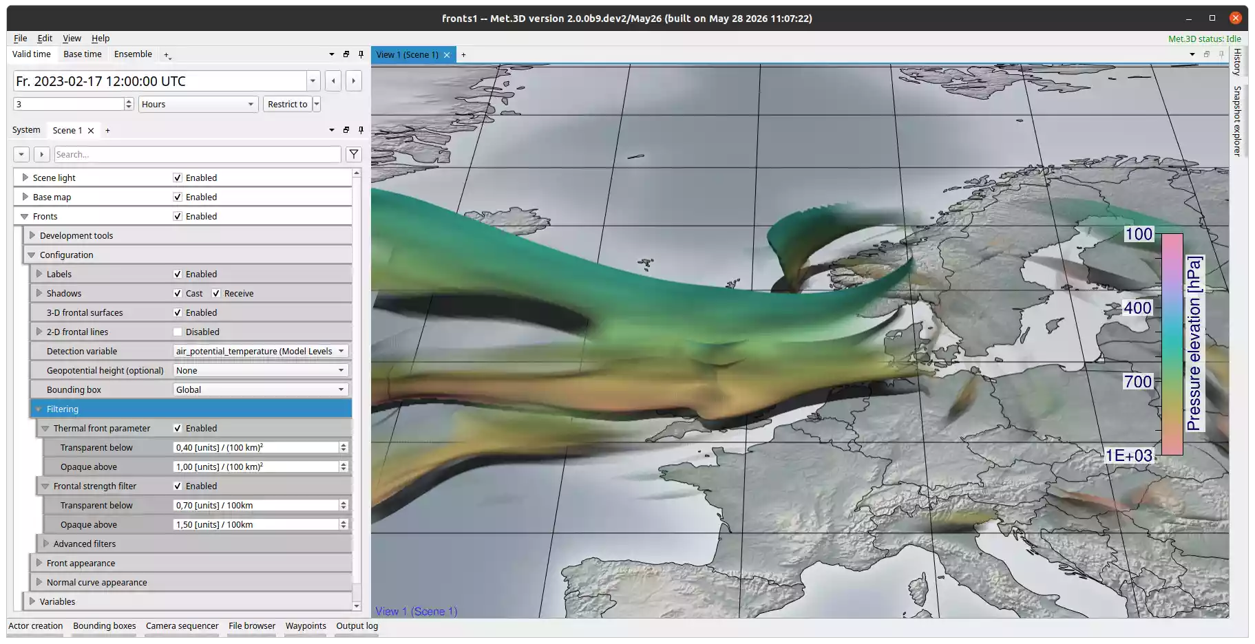
Fig. 40 Front detection actor showing 3-D frontal surfaces.
Description
The front detection actor identifies and visualises atmospheric fronts in 3-D numerical weather prediction data. Both two-dimensional frontal lines at a fixed pressure level and three-dimensional frontal surfaces spanning multiple pressure levels are supported.
The detection method follows Hewson’s front location equation (FLE) approach as described and extended to three dimensions in Beckert et al. (2023). The detection variable (typically equivalent potential temperature or wet-bulb potential temperature) is used to locate fronts by finding zeroes of its third horizontal derivative. A smoothed input field (box blur with a horizontal distance of roughly 100 km) is recommended to avoid visual artefacts and speed up computation.
Note
The actor warns if the detection variable is not smoothed. Smoothing can be configured in the actor variable properties.
Detection pipeline
The front computation pipeline consists of several chained processing steps:
- Front location equation (FLE)
Locates the front by searching for zeroes of the third horizontal derivative of the detection variable (the five-point mean axis of Hewson 1998). The zero-crossing of the FLE field marks the frontal zone.
- Thermal front parameter (TFP)
A measure of front intensity based on the second derivative of the detection variable in the direction of the horizontal gradient. Positive TFP values identify the warm side of the frontal zone; it is used to suppress the cold side of fronts and to filter out weak features. See Fig. 1 of Beckert et al. (2023).
- Adjacent baroclinic zone (ABZ)
An additional masking field following Hewson (1998) that characterises the strength of the baroclinic zone surrounding the front.
- 2-D front lines
The marching squares algorithm is applied to the FLE field at a chosen pressure level. Connected line segments are assembled into front lines, and undersized fragments are discarded. Normal curves are integrated along the thermal gradient at each front line vertex to fill frontal parameters for filtering and shading.
- 3-D frontal surfaces
The marching cubes algorithm is applied to the 3-D FLE field, producing a triangulated surface. Normal curves are computed for each surface vertex on the GPU to derive the frontal parameters used for filtering and shading.
The pipeline first generates the front geometry from the FLE field, then integrates normal curves to fill per-vertex frontal parameters (TFP, ABZ, breadth, slope). The filters (TFP, frontal strength, ABZ, etc.) are not separate processing modules; they act purely as per-vertex alpha masks applied on the GPU during rendering, and changing them does not trigger a pipeline recomputation.
Variables
- Detection variable
The scalar field used for front detection. Equivalent potential temperature or wet-bulb potential temperature are typical choices. The variable should be smoothed (see note above).
- Geopotential height (optional)
If provided, the geopotential height field is used to compute the true geometric slope of 3-D front surfaces. Without it, a standard atmosphere approximation is used.
- Eastward and northward wind components (optional)
Required only when the Map front type colour mode is selected. The wind components are used to determine whether a front is a warm or cold front.
Rendering modes
Enable 3-D frontal surfaces to render the front as a triangulated surface through the full vertical extent of the bounding box.
Enable 2-D frontal lines to render the front at a fixed pressure level as tubes. The Elevation property sets that pressure level (default 850 hPa), and Tube radius controls the tube size.
Both modes can be active simultaneously.
Filtering
All filters control front opacity via a min-max range. Frontal elements with a value below the minimum are fully transparent; above the maximum they are fully opaque; a smooth linear transition occurs in between.
- Thermal front parameter (TFP)
Filters by front intensity. Raising the minimum discards weak fronts. Values are in units of the detection variable per (100 km)².
- Frontal strength
Filters by the gradient magnitude of the detection variable within the frontal zone, in units per 100 km. This controls the minimum thermal contrast required to show a front.
The Advanced filters group provides three additional filters:
- Adjacent baroclinic zone (ABZ)
Filters by the ABZ value following Hewson (1998). Useful for suppressing fronts in regions of weak baroclinicity.
- Breadth of frontal zone
Filters by the horizontal extent of the frontal zone (in km). Can be used to suppress very narrow or diffuse fronts.
- Slope (3-D only)
Filters by the slope of the 3-D front surface. Requires the geopotential height variable to be set.
- Additional variable filters
Click Add additional filter to add filters based on arbitrary actor variables. Each such filter applies a threshold on either the absolute change, the change per 100 km, or the value at the front vertex of the selected variable.
Appearance
The Colour mode setting controls how the frontal surface or lines are coloured:
Constant colour: a single user-defined colour applied uniformly.
Shading variable: colour mapped from an arbitrary actor variable via a transfer function. The variable can be sampled as its absolute change across the frontal zone, its change per 100 km, or its value at the front vertex.
Map pressure: colour encodes the pressure of the front vertex.
Map TFP: colour encodes the thermal front parameter.
Map ABZ: colour encodes the adjacent baroclinic zone value.
Map slope: colour encodes the slope of the 3-D front surface.
Map breadth of frontal zone: colour encodes the frontal zone width.
Map front type: colour encodes whether the front is a warm or cold front. Requires the eastward and northward wind components to be set.
All colour modes except Constant colour and Map front type use a user-defined transfer function to map values to colours.
Normal curves
Normal curves follow the horizontal thermal gradient away from the front and visualise the extent and structure of the frontal zone. They are available in both 2-D (at the chosen elevation) and 3-D.
Tube radius: radius of the rendered normal curve tubes.
Seed point spacing (horizontal): distance between seed points along the front line in degrees. Smaller values produce denser normal curves.
Seed point spacing (vertical): vertical spacing between seed points on a 3-D front surface in hPa.
Colour mode and Mapped variable: equivalent to the front appearance settings above, applied to normal curves independently.
Performance and data resolution
Front detection is computationally expensive, particularly in 3-D mode. On lower-end hardware, consider using a coarser-resolution dataset or restricting the bounding box to a smaller area before enabling 3-D frontal surfaces.
The bounding box also has an important influence on result quality:
Vertical range: the frontal surface is computed across the full vertical extent of the bounding box. Setting the bottom pressure higher than roughly 900 hPa avoids the boundary layer near the surface, where the FLE tends to produce spurious detections over land. The top of the bounding box can typically be set to around 300 hPa, as fronts above that level are uncommon in the mid-latitudes.
Horizontal resolution: at very high grid spacings the third derivative of the detection variable becomes so small that floating-point arithmetic can no longer represent it accurately, leading to numerical artefacts and largely unusable results (e.g. ICON-D2 at ~2.2 km is generally not usable). This is a current limitation of the implementation. Data at roughly 10-30 km grid spacing (e.g. ICON-EU, IFS) works well.
References
Beckert, A. A., Eisenstein, L., Oertel, A., Hewson, T., Craig, G. C., and Rautenhaus, M.: The three-dimensional structure of fronts in mid-latitude weather systems in numerical weather prediction models, Geoscientific Model Development, 16, 4427-4450, https://doi.org/10.5194/gmd-16-4427-2023, 2023.
Hewson, T. D.: Objective fronts, Meteorological Applications, 5, 37-65, https://doi.org/10.1017/S1350482798000553, 1998.